Cracking The Black Box

Introduction to Adversarial Machine Learning Through FGSM

My Journey into Adversarial Machine Learning:

Ever wondered if those clever algorithms recommending your next Netflix binge or recognizing faces at airport security could be tricked? I did too. Machine learning powers so much of our world, yet its vulnerabilities remain largely hidden. We often perceive these AI systems as “black boxes” — mysterious entities that magically produce results. But what if we could peek inside, understand their inner workings, and even manipulate them?

Last year, I dove into this fascinating realm through TAU’s Trustworthy Machine Learning course, and what I discovered was eye-opening: yes, these models can be deliberately fooled, and often with surprising ease. We can, in fact, “crack” that black box.

That course, packed with insightful lectures, hands-on assignments, and deep dives into cutting-edge research, ignited my passion for adversarial machine learning. I want to share that excitement with you, starting with a simple yet powerful attack: the Fast Gradient Sign Method (FGSM). This post marks the beginning of a series where we’ll explore the intricacies of adversarial ML, from practical examples and guides to unexpected discoveries.

Literally cracked box

What is Adversarial Machine Learning?

Adversarial machine learning is a field dedicated to understanding and exploiting the vulnerabilities of machine learning models. It’s a broad discipline encompassing various attack strategies, each designed to compromise the integrity and reliability of AI systems. These attacks manifest in numerous forms, including:

• Poisoning Attacks: Where malicious data is injected into training sets, corrupting the model’s learning process from the ground up.

• Model Extraction Attacks: In which attackers attempt to clone a model’s functionality by repeatedly querying it, effectively stealing its learned knowledge.

• Backdoor Attacks: That embed hidden triggers within models, causing them to behave maliciously only when specific conditions are met.

• Evasion Attacks: Which focus on manipulating inputs during the model’s operational phase to cause misclassifications or errors.

These attacks pose significant risks to real-world applications of machine learning, from self-driving cars misinterpreting traffic signals to medical AI misdiagnosing patients. The potential for disruption and harm is vast, underscoring the importance of understanding these vulnerabilities.

Within this diverse landscape of attacks, adversarial examples stand out as a particularly compelling and accessible area of study. These are meticulously crafted inputs designed to deceive machine learning models during inference. Think of them as finding and exploiting the model’s blind spots.

In this post, we’ll delve into the creation and implications of adversarial examples, using the Fast Gradient Sign Method (FGSM) as our primary tool. This exploration will serve as an entry point into the broader field of adversarial machine learning.

What is an adversarial example?

“Adversarial examples are specialized inputs designed to intentionally mislead machine learning models, leading to misclassifications. As TensorFlow’s guide aptly puts it, these “notorious inputs are indistinguishable to the human eye, but cause the network to fail to identify the contents of the image.”

One of the most iconic demonstrations of this phenomenon comes from Goodfellow et al.’s paper, ‘Explaining and Harnessing Adversarial Examples’, which showcased how subtle perturbations could drastically alter a model’s predictions.

To better understand the landscape of adversarial attacks, we can categorize them along a few key dimensions:

• Targeted vs. Untargeted Attacks: There are different goals when attacking ML model. An ‘untargeted attack’ simply aims to make the model get it wrong. A ‘targeted attack’ aims to make the model misclassify the input as a specific, chosen thing.

• White-Box vs. Black-Box Attacks: Attacks also differ in how much information the attacker has. A ‘white-box attack’ means the attacker knows everything about the model. A ‘black-box attack’ means the attacker only sees the inputs and outputs.”

The following attack, will be White-Box, untargeted attack.

Quick Reminder — Image Classification

To understand how adversarial attacks work, let’s revisit the fundamental task of image classification. Imagine training a model to recognize objects in photographs. This model takes an image as input and produces a prediction, which is a label indicating the model’s interpretation of the image’s content.

For our demonstration, we’ll use the vit-base-patch16-224 Vision Transformer, a model pre-trained on a vast dataset of images. This model is capable of classifying images into 1000 distinct categories.

Consider this image of a cute beagle:

Cute beagle

When we feed this image to the vit-base-patch16-224 model, we obtain the following classification results:

Base Image classification on huggingface, we got great beagle deteactor!

As you can see, the model outputs a probability distribution over the 1000 possible classes, with “beagle” receiving the highest probability.

In order to attack, we will need to get to use code, here is a simple snippet to do it (you can copy do it in your own environment or Colab notebook):

import torch
import matplotlib.pyplot as plt
from PIL import Image
import requests
import io
from transformers import AutoModelForImageClassification, AutoImageProcessor

MODEL_NAME = "google/vit-base-patch16-224"
IMAGE_URL = "https://images.unsplash.com/photo-1543466835-00a7907e9de1?auto=format&fit=crop&w=224&h=224"

model = AutoModelForImageClassification.from_pretrained(MODEL_NAME)
image_processor = AutoImageProcessor.from_pretrained(MODEL_NAME)

image = Image.open(io.BytesIO(requests.get(IMAGE_URL).content)).convert("RGB")
processed_image_tensor = image_processor(images=image, return_tensors="pt").pixel_values

logits = model(processed_image_tensor).logits
predicted_class_idx = logits.argmax(-1).item()
predicted_class = model.config.id2label[predicted_class_idx]
confidence = torch.softmax(logits, dim=1)[0][predicted_class_idx].item()

plt.figure(figsize=(12, 6))
plt.subplot(1, 2, 1)
plt.imshow(image)
plt.title(f"Label: {predicted_class} \nConfidence: {confidence:.2f}")
plt.axis('off')

plt.show()

The expected Output

While we won’t delve into the intricate details of the model’s architecture, it’s essential to understand the basic process. The image is first transformed into a tensor, a multi-dimensional array of numerical values. This tensor then passes through a series of layers within the Vision Transformer. Each layer performs computations that extract increasingly abstract features from the image. Finally, the output layer produces the probability distribution over the class labels.

During the model’s training, it learned to recognize images by repeatedly receiving images, calculating the loss (the difference between its predictions and the correct labels), and using the gradients of that loss to adjust its internal parameters. In essence, it used gradients to improve its accuracy. Now, we are going to exploit those very same gradients, not to improve the model, but to trick it. By manipulating the input image based on the gradients.

Unveiling the Attack: The Fast Gradient Sign Method (FGSM)

Now that we’ve seen how our vit-base-patch16-224 confidently classifies our beagle image, let’s explore how to create an adversarial example using the Fast Gradient Sign Method (FGSM). Remember, we’re focusing on an untargeted attack, meaning we want to make the model misclassify the image, regardless of the specific incorrect label it chooses.

The Fast Gradient Sign Method (FGSM) works by leveraging the gradients of the neural network to craft an adversarial example. Specifically, it uses the gradients of the loss function with respect to the input image to generate a perturbed image that maximizes the loss. This perturbed image is our adversarial example, designed to fool the model.

Here’s a breakdown of the process:

1. Calculate the Loss: We feed the original image into the model and calculate the loss between the model’s prediction and the true label. In our untargeted attack, we will use the loss of the predicted label.

2. Compute the Gradients: We then compute the gradients of the loss with respect to the input image. These gradients reveal how each pixel’s change affects the loss for the predicted class.

3. Take the Sign of the Gradients: We take the sign of each gradient (+1 or -1) to determine the direction of perturbation.

4. Apply Perturbation: We multiply the sign of the gradients by a small value called epsilon (ε) and add it to the original image. Epsilon controls the magnitude of the perturbation.

Mathematically, FGSM can be expressed as:

where

• x’ : Adversarial image.

• x : Original input image.

• y : Original input label.

• ϵ : Multiplier to ensure the perturbations are small.

• θ : Model parameters.

• J : Loss.

This method is computationally efficient because we can easily find these gradients using the chain rule. It’s important to note that during this attack, the model parameters (θ) remain constant. We are not training the model; we are simply exploiting its existing vulnerabilities to generate an adversarial example.

Essentially, we’re nudging the image in the direction that makes the model most confident about the wrong answer. In the next section, we will see how this translates into code.

FGSM implementation

def calculate_gradients(input_tensor):
    input_tensor_copy = input_tensor.detach().clone().requires_grad_(True)
    logits = model(input_tensor_copy).logits
    original_prediction_index = torch.argmax(logits, dim=1).item()
    loss = logits[0, original_prediction_index]
    self.model.zero_grad()
    loss.backward()
    return input_tensor_copy.grad.data.sign()

def calculate_adversarial_tensor(input_tensor):
    gradients = calculate_gradients(input_tensor)
    return (input_tensor + EPSILON * gradients.sign()).clamp(-1, 1)

Let’s break down these functions:

• calculate_gradients: This calculates the gradients of the loss with respect to the input. It makes a copy of the input tensor, gets the model’s logits on it, finds the predicted class index, calculates the loss, performs backpropagation to get the gradients, and returns the negation of the sign of the gradients (I’m sorry for all of the big words, I added links if you are not sure about the meaning).

• calculate_adversarial_tensor: This function creates the adversarial tensor. It calls calculate_gradients to get the gradients, adds the perturbation (epsilon times the sign of the gradients), and uses clamp to ensure pixel values stay within -1 and 1.

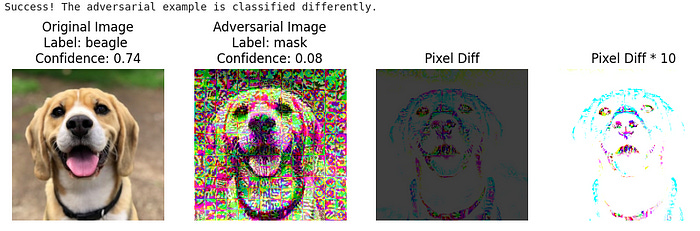
After adding the remaining code (model loading, preprocessing, visualization), which can be found in the Colab notebook, you’ll obtain the folliwing adversarial image:

SUCSSES!

We made it! The model now thinks that the dog is actually Labrador retriever and the image looks almost the same for us.

Might be Little bit anticlamatic but don’t have much control in the untargeted attack. Spoiler: In the next post we will use targeted attack and we will be able to make the model think that the model is cat, panda or whatever.

Epsilon and Its Role

A critical parameter in FGSM is ϵ. It dictates the magnitude of the perturbation we apply to the image.

• A small epsilon results in a subtle perturbation, making the adversarial example harder to detect.

• A large epsilon leads to a more noticeable perturbation, potentially making the attack more effective but also easier to spot.

Experimenting with different epsilon values can reveal the trade-off between attack strength and stealth.

For example, if we run the previous experiment with different epsilon values we will get different results, Lets see that:

Fail! Epsilon= 0.0001

Success! Epsilon = 0.05

Very Noisy (and probably unwanted) Success! Epsilon = 0.5

We can see that different values yields completely different results, choosing the correct values depends on the context. You can try more images and epsilon in the Colab notebook

Conclusion and Further Exploration

The FGSM attack provides a compelling illustration of the vulnerabilities inherent in machine learning models. By understanding these vulnerabilities, we can begin to develop more robust and trustworthy AI systems.

I hope this post has given you a taste of the fascinating world of adversarial machine learning. But we’ve only scratched the surface! In future posts, we’ll delve deeper into more advanced attack techniques and explore the exciting realm of defenses.

Specifically, we’ll cover:

• Targeted FGSM: Where we aim to make the model misclassify an image as a specific chosen label.

• Targeted Projected Gradient Descent (PGD): A powerful iterative attack that often surpasses FGSM in effectiveness.

• Adversarial Attacks on Audio: Exploring how similar principles can be used to manipulate audio signals and fool speech recognition systems.

• Adversarial training: How the adversarial examples could be used in the training process to make models that are not only more robust, but more precise in general.

• And much more!

I’m eager to hear from you! What aspects of adversarial machine learning are you most interested in? What topics would you like to see covered in future posts? Your feedback will help shape the direction of this series. Let’s continue this journey of cracking the black box together!